Learning jQuery in 30 minutes
View more presentations from simon.
DBCC SHRINKDATABASE (dbName)DBCC SHRINKFILE (logicalLogFileName)USE dbName
EXEC sp_helpfile/* Shrink Whole AdventureWorks Database */
DBCC SHRINKDATABASE (AdventureWorks)
GO
/* Get the Logical File Name */
USE AdventureWorks
EXEC sp_helpfile
GO
/* Shrink MDF File of AdventureWorks Database */
DBCC SHRINKFILE (AdventureWorks_Data)
GO
In this tip series I've covered many aspects of datetime values in SQL Server. The examples I have shown you were written for SQL Server 2005, though much of what I discussed in those articles could also apply to SQL Server 2008. In this tip, I take the discussion of datetime values one step further and focus specifically on the new datetime data types available in SQL Server 2008. They include the DATE, TIME, DATETIME2 and DATETIMEOFFSET types as they're supported in Transact-SQL.
To demonstrate these types, I use the following code to create the Sales.OrderDates table in the AdventureWorks2008 sample database and to insert test data into the table:
USE AdventureWorks2008
GO
IF EXISTS (SELECT table_name
FROM information_schema.tables
WHERE table_schema = 'Sales'
AND table_name = 'OrderDates')
DROP TABLE Sales.OrderDates
GO
CREATE TABLE Sales.OrderDates
(
OrderID INT NOT NULL,
Date_Type DATE NULL,
Time_Type TIME(7) NULL,
DateTime2_Type DATETIME2(7) NULL,
DateTimeOffset_Type DATETIMEOFFSET(7) NULL
)
GO
INSERT INTO Sales.OrderDates
VALUES(1001, '2008-09-22', '18:27:10.1234567',
'2008-09-22 18:27:10.1234567', '2008-09-22 18:27:10.1234567 -07:00')
If you want to try out the examples in this article, you can create the table in the AdventureWorks2008 database or in a different database. If you decide to use the AdventureWorks2008 database, the necessary files are available from CodePlex.
The DATE data type
Prior to SQL Server 2008, the primary datetime data types were DATETIME and SMALLDATETIME. In each case, the value stored in the type contained both the date and time, and there was no way to store one portion without the other. However, SQL Server 2008 changes all that with the DATE and TIME data types.
As the name suggests, the DATE data type stores a date value. The value can range from January 1, 1 A.D. through December 31, 9999 A.D. The value includes the year, month and day. For example, the following SELECT statement retrieves data from the OrderID and Date_Type columns:
SELECT OrderID, Date_Type FROM Sales.OrderDates
The Date_Type column is configured with the DATE data type, so the value returned contains only a date, as in the following results:
| OrderID | Date_Type |
| 1001 | 2008-09-22 |
If you want to return a datetime value as a DATE value, you can explicitly convert the value, as in the following SELECT statement:
SELECT OrderID, CAST(DateTimeOffset_Type AS DATE) AS ConvertedType
FROM Sales.OrderDates
In this case, the statement retrieves the value from the DateTimeOffset_Type column, which is configured with the DATETIMEOFFSET data type (explained later in the article). This statement returns the same results as those returned by the previous statement, even though the retrieved value contains both date and time data. In other words, the time portion of the value is ignored.
When inserting data into a DATE column, you can specify a date value or a datetime value, as shown in the following example:
INSERT INTO Sales.OrderDates (OrderID, Date_Type)
VALUES (1002, '2008-09-20');
INSERT INTO Sales.OrderDates (OrderID, Date_Type)
VALUES (1003, '2008-09-21 18:27:10.1234567');
When you specify a datetime value, SQL Server automatically converts that value into the DATE data type, which means that only the date portion is stored.
The TIME data type
The TIME data type stores only the time value. The value itself supports a fractional precision of 7. This means that the fractional part of the seconds can support up to seven decimal places, compared to a DATETIME value, which has a fractional precision of 3. The precision of the TIME data type supports a range of 00:00:00.0000000 through 23:59:59.9999999.
When you specify the TIME data type in a Transact-SQL statement, you can specify the precision of the stored values by including the appropriate number within parentheses. For example, to specify a precision of 7, you would specify TIME(7). For a precision of 5, you would specify TIME(5), and so on. If you do not specify the precision, 7 is assumed.
The TIME data type returns data in the form of hour, minute, second and fractional second. For instance, the following SELECT statement retrieves data from the Time_Type column:
SELECT OrderID, Time_Type FROM Sales.OrderDates
The Time_Type column is configured with the TIME(7) data type, so it returns data in the following form:
| OrderID | Time_Type |
| 1001 | 18:27:10.1234567 |
Notice that the column returns only the time and that the value has a fractional precision of 7.
As you saw with the DATE data type, you can also return a TIME value from a datetime column. For example, the following statement retrieves data from the DateTimeOffset_Type column and converts the value to TIME(7):
SELECT OrderID, CAST(DateTimeOffset_Type AS TIME(7)) AS ConvertedType
FROM Sales.OrderDates
The SELECT statement returns the same results as the previous SELECT statement.
You can, however, specify a different precision when converting the data, as shown in the following example:
SELECT OrderID, CAST(DateTimeOffset_Type AS TIME(5)) AS ConvertedType
FROM Sales.OrderDates
The fractional part of the seconds now includes only five decimal places:
| OrderID | ConvertedType |
| 1001 | 18:27:10.12346 |
Notice that the fractional seconds have been rounded up. The original fractional seconds were .1234567. However, if you specify a precision of 5, SQL Server will round up the "67" fractional part, returning .12346 in the results, rather than .12345.
As with a DATE column, when inserting data into a TIME column, you can specify a time value or a datetime value as shown in the following INSERT statements:
INSERT INTO Sales.OrderDates (OrderID, Time_Type)
VALUES (1004, '18:27:10.1234567');
INSERT INTO Sales.OrderDates (OrderID, Time_Type)
VALUES (1005, '2008-09-20 18:27:10.1234567');
In both cases, only the time is inserted into the Time_Type column.
The DATETIME2 data type
The DATETIME2 data type is similar to the DATETIME data type. The difference is that DATETIME2 supports a wider range of dates (same as DATE) and a greater fractional precision (same as TIME). And like the TIME data type, you can specify that precision.
In other words, the DATETIME2 data type basically combines a DATE value and a TIME value. For example, the following SELECT statement returns data from the DateTime2_Type column, which is configured as a DATETIME2 column:
SELECT OrderID, DateTime2_Type FROM Sales.OrderDates
The statement returns the following results:
| OrderID | DateTime2_Type |
| 1001 | 2008-09-22 18:27:10.1234567 |
As you can see, the DATETIME2 value first provides the date, then the time, with a fractional precision of 7. Except for the seven digits of the fractional seconds, this value looks just like a DATETIME value –or a DATE valued followed by a TIME value.
You can also convert other datetime values to a DATETIME2 value, as in the following statement:
SELECT OrderID, CAST(DateTimeOffset_Type AS DATETIME2(7)) AS ConvertedType
FROM Sales.OrderDates
Notice that I'm converting a DATETIMEOFFSET value to DATETIME2 and that I'm specifying a precision of 7. This statement will return the same results as the previous statement.
But the results are quite different if you convert other types of values. For instance, the following statement retrieves data from the Date_Type column, which is configured with the DATE data type and converts the value to DATETIME2(7):
SELECT OrderID, CAST(Date_Type AS DATETIME2(7)) AS ConvertedType
FROM Sales.OrderDates
When SQL Server converts the value, it adds a default time to the new value, as shown in the following results:
| OrderID | ConvertedType |
| 1001 | 2008-09-22 00:00:00.0000000 |
Notice that the time is all zeroes (with a precision of 7), which is the first value of the 24-hour clock. Whenever the time needs to be assumed (as in this case), all zeroes are used, which means that the default time value is 00:00:00.0000000.
The default value for the date is quite different. In the following statement, I convert the value from the Time_Type column, which is configured with the TIME data type, to a DATETIME2(7) value:
SELECT OrderID, CAST(Time_Type AS DATETIME2(7)) AS ConvertedType
FROM Sales.OrderDates
Because no date is included in a TIME value, SQL Server assumes a date, as shown in the following results:
| OrderID | ConvertedType |
| 1001 | 1900-01-01 18:27:10.1234567 |
As you can see, the date is January 1, 1900. This is the default date when no date is provided.
If a picture is worth a thousand words, then a free data modeling tool is worth a terabyte of data. That is just what you get with the SQL Server 2000 DaVinci data modeling tools. SQL Server 2000 Enterprise Manager has a number of hidden goodies, and the DaVinci tools seem to elude more DBAs and developers than just about any other feature.
A data model is a visual representation of the physical tables, columns, data types, lengths, null value and referential integrity. The DaVinci tools are a basic set of visual data modeling tools used to build a data model and support a basic data dictionary, which defines all of the tables, columns and relationships that exist in the data model.
I am surprised by the number of DBAs and developers I've worked with who do not know that data modeling features exist natively in SQL Server. Their eyes light up when they get a data model, which they refer to as "wall paper." Their walls may be covered with data models from other systems that they have talked about for months or years, but never really seen. Now the are able to visually identify issues that have been floating around in their heads.
If you are already using the DaVinci tools or a product from another vendor, I commend you. I think data models are underutilized in achieving high performance. They serve as common ground between the users and other members of the IT team that need to migrate data or generate reports. These additional benefits will convince the rest of you non-users about the value of data models:
The following is important to keep in mind so you do not lose data. When you change the data model (i.e. your pretty picture in Enterprise Manager), you are changing your database. Take care when you make the changes in your development environment, script out the changes, save the changes to a text file and apply the changes to the production environment during a maintenance window.
In situations where the tables have data, under-the-covers the DaVinci tools create a temporary table, issue a SELECT INTO statement into the temporary table, drop the current table and rename the temporary table to the original table name. This set of processing is not what you want to occur on your production environment during the middle of the day.
The DaVinci tools are very simple to use, but if you do not understand how they work you can have serious problems.
You can access the DaVinci tools in Enterprise Manager 2000 by navigating to the SQL Server, opening the Databases folder, expanding the individual database, left clicking on the Diagrams folder and right clicking on the right pane to select the New Database Diagram option. Table 1 below outlines the steps the wizard will follow:
| Directions | |
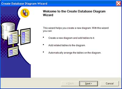 | After reviewing the directions, click the 'Next' button to proceed with the Create Database Diagram Wizard. |
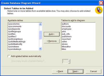 | From the 'Available tables' in the left pane, press the 'Add' button to include the tables in the 'Tables to add to diagram' pane on the right. Press the 'Next' button to proceed with the wizard. |
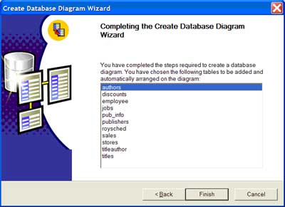 | Press the 'Finish' button to complete the wizard and have SQL Server automatically arrange the tables. |
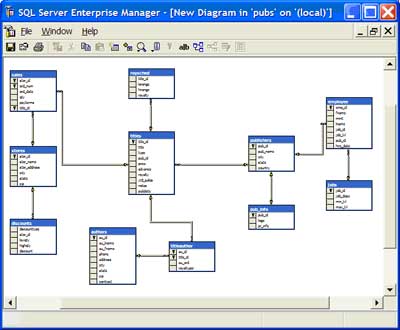 | The tables are automatically arranged on the canvas. The data model outlines the primary keys with a golden key and the foreign keys with a connecting line between the tables. |
Table 1: New database diagram
Once the data model is built, be prepared to use the DaVinci tools' core functionality (shown in Table 2).
| ID | Functionality | Directions | Screen shot |
| 1 | Save the data model | On the top left portion of the interface, click the 'Disk' icon on the toolbar to save the data model. The first time the data model is saved, you will be prompted to name the data model. This is shown in the graphic to the right. | 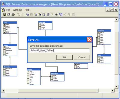 |
| 2 | Change the view of the data model | On the toolbar, select the 'Show' icon to determine which level of detail you would like displayed in the data model. I typically like to use the 'Standard' option because I am able to see the table name, column name, primary key, data type, length and null property | 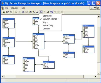 |
| 3 | Add a comment to the data model | On the toolbar, select the 'New Text Annotation' icon to add text to the data model. I typically like to add comments for particular groups of tables as well as notes for the data model (i.e., date, developer, database, project, etc.). | 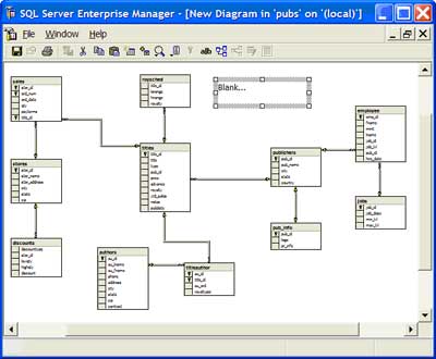 |
| 4 | Add an existing table to the data model | On the toolbar, select, 'Add table to Diagram' icon to add an existing table. Scroll to find the table you want to add and then press the 'Add' button to add the table to the data model. If the table has a primary key or any referential integrity to other tables, this will appear on the model. | 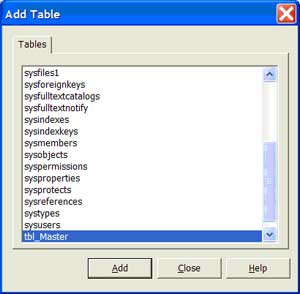 |
| 5 | Add a new table to the data model | On the toolbar, select, the 'New Table' icon to add a table that has not existed in the database. First name the table. Second add the columns, primary key, etc., for the table as outlined below. | 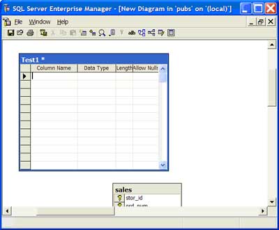 |
| 6 | Add a column, which is really a row in one of the tables in the data model | Navigate to the table where the column should be added. Right click on the row. Select the 'Insert Column' option. Fill-in the 'Column Name,' 'Data Type,' 'Length' and 'Allow Nulls' properties. | 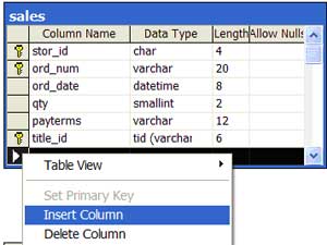 |
| 7 | Remove a column in a table, which is actually a row | Navigate to the table where the column should be removed. Right click on the row. Select the 'Delete Column' option. The column will be deleted without confirmation. | 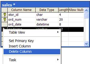 |
| 8 | Assign a primary key to a table | Right click on the column name and select the 'Set Primary Key' option. A golden key will appear to the left of the column name. | 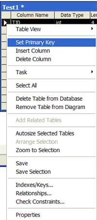 |
| 9 | Build a primary key foreign key relationship | Drag and drop the primary key column to the foreign key column by holding down the left mouse button. | 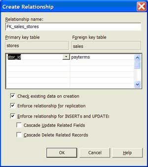 |
| 10 | Remove a table from the diagram versus delete the table from the diagram | The 'Remove Table from Diagram' option retains the table in the database, but it is removed from the model. The 'Delete Table from Database' permanently destroys the table. To access this functionality, navigate to the table, right click on the table and select either 'Remove Table from Diagram' or 'Delete Table from Database' option. |  |
Table 2: Add functionality to the database.
A hidden feature within the DaVinci tools is the ability to generate a basic data dictionary. Table 3 shows the primary screens for completing these tasks.
| ID | Functionality | Directions | Screen shot |
| 1 | Add a table definition | Right click on the table and select 'Properties' to access the interface. Type in the table description on the 'Tables' tab in the 'Description' text box. | 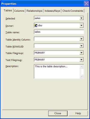 |
| 2 | Add a column definition | Right click on the table and select 'Properties' to access the interface. Type in the column description on the 'Columns' tab in the 'Description' text box. | 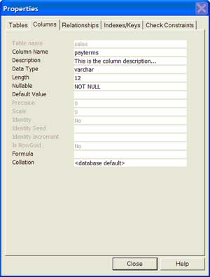 |
Table 3: Add table and column definitions.
Once you have entered all the table descriptions, execute the following query to access all table-level definitions:
SELECT o.id AS 'ObjectID',
CAST(o.Name AS varchar(25)) AS 'TableName',
CAST(p.Value AS varchar(50)) AS 'Description'
FROM dbo.sysobjects o
INNER JOIN dbo.sysproperties p
 ON o.id = p.id
WHERE p.type = 3
AND p.smallid = 0
ORDER BY o.id, o.Name
Once you have entered all table and column descriptions, execute the following query to access table and column definitions:
SELECT o.id AS 'ObjectID',
CAST(o.Name AS varchar(25)) AS 'TableName',
CAST(c.Name AS varchar(25)) AS 'ColumnName',
CAST(p.Value AS varchar(50)) AS 'Description',
Type = CASE WHEN p.Type=3 THEN 'Table' WHEN p.Type=4 THEN 'Column' ELSE 'UNKNOWN' END
FROM dbo.sysobjects o
INNER JOIN dbo.sysproperties p
 ON o.id = p.id
INNER JOIN dbo.syscolumns c
 ON p.smallid = c.colorder
WHERE o.id = c.id
AND p.type = 4
ORDER BY o.id, o.Name, p.smallid
To help you prepare for new options in SQL Server 2005, available in November 2005, I highly recommend leveraging the DaVinci tools in SQL Server 2000 if you are not already using a data modeling tool. Among other improvements, I hope the printing capabilities improve to distribute the data model as well as the representation of the primary key and foreign key relationships so that the connecting lines are relative between the two columns rather than two tables. Although these are minor points, hopefully this functionality and other aspects of the tool will be greatly improved with SQL Server 2005. Stay tuned!
About the author: Jeremy Kadlec is the Principal Database Engineer at Edgewood Solutions, a technology services company delivering professional services and product solutions for Microsoft SQL Server. He has authored numerous articles and delivers frequent presentations at regional SQL Server Users Groups and nationally at SQL PASS. Jeremy is also the SearchSQLServer.com Performance Tuning expert. Ask him a question here.
Performance tuning is not easy and there aren’t any silver bullets, but you can go a surprisingly long way with a few basic guidelines.
In theory, performance tuning is done by a DBA. But in practice, the DBA is not going to have time to scrutinize every change made to a stored procedure. Learning to do basic tuning might save you from reworking code late in the game.
Below is my list of the top 15 things I believe developers should do as a matter of course to tune performance when coding. These are the low hanging fruit of SQL Server performance – they are easy to do and often have a substantial impact. Doing these won’t guarantee lightening fast performance, but it won’t be slow either.
If you take these 15 steps, you’ve made a really good first pass.
There’s more to learn next time as we build a model of how your application, the network, and SQL Server all offer the potential for bottlenecks. We will also look at the potential for improving performance and some more steps that you can take without stepping too far into the land of the DBA